Stage 5: Trait Extraction¶

Extract scale-invariant plant trait signals from the canonical 3DGS render, for relative growth monitoring across sessions.

Monitoring, not absolute measurement

The traits below (h_norm, a_norm) are normalized, scale-invariant quantities intended to track change over time and detect events (e.g. pruning). They are not calibrated absolute heights/areas — consistency across sessions (CV) is the metric that matters. See Results & Validation.

What This Stage Does¶

graph LR
    A[🎥 3DGS Model<br/>per session] -->|Render pose 025| B[📷 Canonical Image<br/>1600×899 px]
    B -->|HSV threshold| C[🌿 Plant Mask]
    C -->|5th–95th percentile| D[📊 h_norm · a_norm]
    style A fill:#e1f5ff
    style D fill:#e1ffe1

Estimated time: ~3 minutes per session (GPU render + analysis)

The Core Innovation¶

Traditional PLY-based methods measure directly in 3D coordinate space — but COLMAP assigns different scales to each date's reconstruction. This makes direct comparison across dates unreliable.

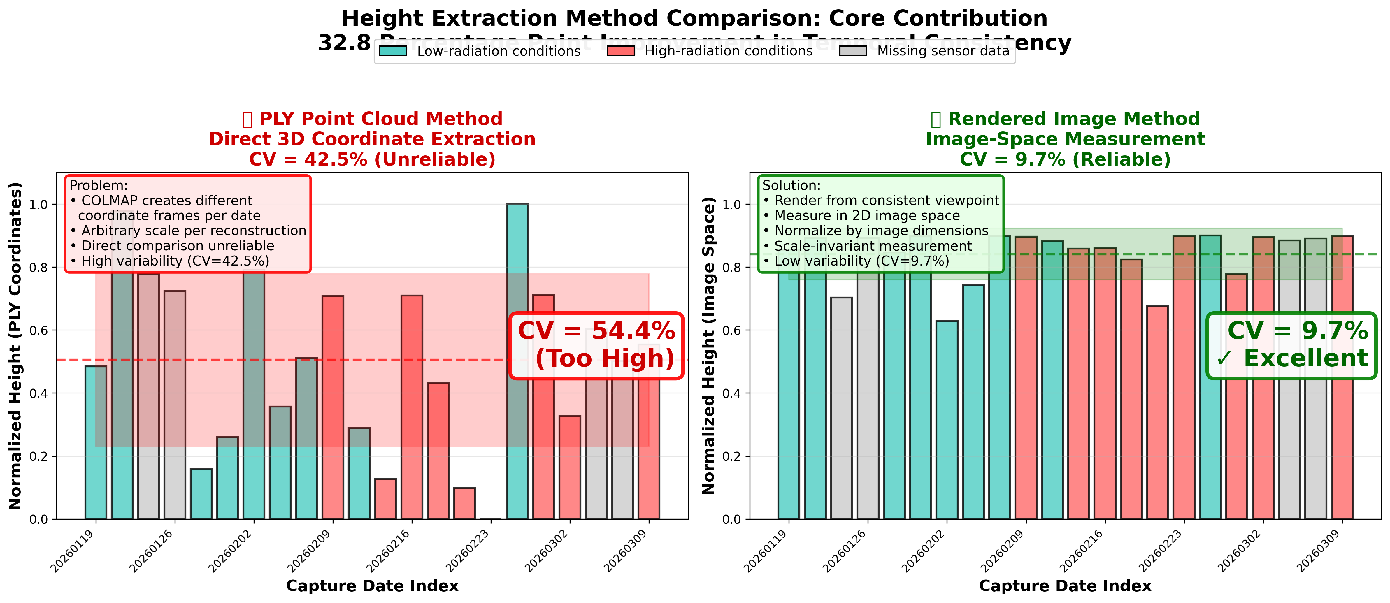Diagram showing scale shift problem in PLY coordinates vs consistency in image space Scale inconsistency: PLY-based height (left) shows erratic shifts between dates. Our image-space method (right) is stable across all 22 dates.

Our solution: synthesise a canonical novel-view image at the fixed canonical pose — the 25^th held-out test frame (the test split keeps every 8^th frame) = cameras.json[200] = frame_00201, ≈40 s into the walk at 5 fps — using the 3DGS renderer, then read plant height in pixel space. The ratio cancels any COLMAP scale factor.

Step 1: Render the Canonical View¶

Use the 3DGS renderer to synthesise the plant from camera pose 025 — the same physical viewpoint across all 22 sessions.

import json, sys, numpy as np, torch
from argparse import Namespace
sys.path.insert(0, '/path/to/gaussian-splatting')
from gaussian_renderer import render, GaussianModel
from utils.graphics_utils import getWorld2View2, getProjectionMatrix

# Load camera pose 025 at native resolution
with open('output/YYYYMMDD/gs_model/cameras.json') as f:
    cam = json.load(f)[200]  # canonical pose = 25th held-out test frame = frame_00201 (~40 s)

W, H = cam['width'], cam['height']
R = np.array(cam['rotation'], dtype=np.float64)
C = np.array(cam['position'], dtype=np.float64)
T = (-R @ C).astype(np.float32)
FoVx = 2 * np.arctan(W / (2 * cam['fx']))
FoVy = 2 * np.arctan(H / (2 * cam['fy']))

Why pose 025?

The canonical pose is the 25^th held-out test frame (the test split keeps every 8^th COLMAP-registered frame). In the full sequential camera list this is cameras.json[200] = frame_00201, ≈40 s into the walk at 5 fps — a view of the crop lane that is fixed once and reused for all 22 sessions. It is rendered as test/ours_30000/renders/00025.png, which is why it is labelled "pose 025".

Step 2: Plant Segmentation (HSV Thresholding)¶

Segment plant from background using HSV colour thresholding.

import cv2
import numpy as np

def segment_plant(img_rgb: np.ndarray) -> np.ndarray:
    """
    Segment green vegetation. Returns binary mask (255 = plant).
    HSV thresholds (OpenCV convention, 8-bit):
      Hue  : [25, 95]   (degrees / 2)
      Sat  : >= 20
      Val  : >= 30
    """
    img_bgr = cv2.cvtColor(img_rgb, cv2.COLOR_RGB2BGR)
    hsv     = cv2.cvtColor(img_bgr, cv2.COLOR_BGR2HSV)
    mask    = cv2.inRange(hsv,
                          np.array([25,  20,  30]),   # lower bound
                          np.array([95, 255, 255]))   # upper bound
    return mask

Threshold values matter

The thresholds above match the published paper exactly (§3.3). Earlier versions of this manual showed different values ([25,40,40]–[90,255,255]) — those are incorrect. Use the values above.

Step 3: Scale-Invariant Height Extraction¶

Measure plant height as a ratio of image height using 5^th–95^th-percentile rows.

def extract_traits(mask: np.ndarray) -> dict:
    """
    h_norm  = (r95 - r5) / H_R    (5th–95th-percentile row span)
    a_norm  = green_pixel_count / (H_R * W_R)
    Both are in [0, 1] and scale-invariant.
    """
    H, W = mask.shape
    plant_rows = np.where(mask.any(axis=1))[0]

    if len(plant_rows) == 0:
        return {"h_norm": 0.0, "a_norm": 0.0, "valid": False}

    r5  = float(np.percentile(plant_rows, 5))
    r95 = float(np.percentile(plant_rows, 95))

    h_norm = (r95 - r5) / H
    a_norm = float(mask.sum()) / 255.0 / (H * W)

    return {
        "h_norm":     round(h_norm, 4),
        "a_norm":     round(a_norm, 4),
        "height_px":  round(r95 - r5, 1),
        "top_row_px": round(r5, 1),
        "bot_row_px": round(r95, 1),
        "image_H":    H,
        "image_W":    W,
        "valid":      True,
    }

Why 5^th–95^th percentile instead of min/max?

Min/max rows are sensitive to isolated green pixels (e.g. stray leaves, reflections). The 5^th–95^th percentile gives a robust estimate of the plant's vertical extent while ignoring outliers.

Step 4: Run for All 22 Sessions¶

The full reproducibility script is analysis/compute_heights_rendered.py. It loops over all sessions, renders from pose 025, and writes analysis/heights_rendered.csv.

conda activate gaussian_splatting

python analysis/compute_heights_rendered.py
# optional: process a subset
python analysis/compute_heights_rendered.py --dates 20260119 20260123
# optional: different output path
python analysis/compute_heights_rendered.py --output results/heights_rendered.csv

Expected output:

Processing 22 sessions → analysis/heights_rendered.csv
Camera: COLMAP index 200  |  Iteration: 30000
HSV thresholds: H∈[25,95], S≥20, V≥30

  20260119  rendering ...  h_norm=0.8990  green_coverage=0.9312  [ok]
  20260121  rendering ...  h_norm=0.8932  green_coverage=0.9584  [ok]
  20260123  rendering ...  h_norm=0.7030  green_coverage=0.7063  [ok]
  ...

Summary (22 sessions):
  h_norm:         mean=0.8432  std=0.0826  CV=9.8%
  green_coverage: mean=0.8653  std=0.1447  CV=16.7%

Results¶

Height CV Comparison¶

Method	CV	vs Proposed
Proposed (render-space h_norm)	9.8%	—
Direct PLY height	28.0%	2.86× worse
Scale-calibrated PLY	35.1%	3.58× worse
Raw-frame baseline	0.0%	(trivial — same image every session)

What 9.8% CV means

The render-space h_norm varies by 9.8% across 22 sessions. Three known pruning events each cause drops of 15–27 percentage points — well above the background variation — confirming the method is sensitive to real biological change, not just measurement noise.

Output CSV Format (`heights_rendered.csv`)¶

date,height_px,height_norm,green_coverage,top_row_px,bottom_row_px,image_H,image_W,status
20260119,808.2,0.8990,0.9312,44.9,853.1,899,1599,ok
20260123,632.0,0.7030,0.7063,235.0,867.0,899,1600,ok

Column	Description
`height_norm`	h_norm — (r95−r5) / H_R, scale-invariant plant height
`green_coverage`	a_norm — green pixel fraction, scale-invariant projected area
`top_row_px` / `bottom_row_px`	r5 / r95 pixel rows
`image_H` / `image_W`	native render resolution from cameras.json

Next: See Full Research Results¶

→ My Research: Original Contributions → Results & Validation